GMM (Gaussian Mixture Model)

GMM is a generative probabilistic model over the contextual embeddings. The model assumes that contextual embeddings are generated from a mixture of underlying Gaussian components. These Gaussian components are assumed to be the topics.

Components of a Gaussian Mixture Model
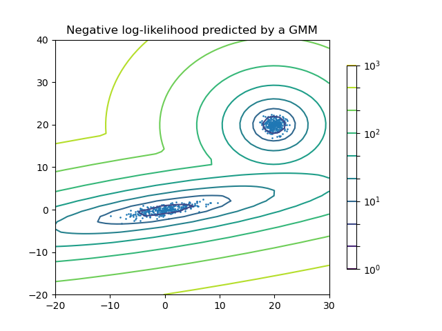
(figure from scikit-learn documentation)

How does GMM work?

Generative Modeling

GMM assumes that the embeddings are generated according to the following stochastic process from a number of Gaussian components. Priors are optionally imposed on the model parameters. The model is fitted either using expectation maximization or variational inference.

Click to see formula

1. Select global topic weights: \(\Theta\)
2. For each component select mean \(\mu_z\) and covariance matrix \(\Sigma_z\) .
3. For each document:
   • Draw topic label: \(z \sim Categorical(\Theta)\)
   • Draw document vector: \(\rho \sim \mathcal{N}(\mu_z, \Sigma_z)\)

Calculate Topic Probabilities

After the model is fitted, soft topic labels are inferred for each document. A document-topic-matrix (\(T\)) is built from the likelihoods of each component given the document encodings.

Click to see formula

• For document \(i\) and topic \(z\) the matrix entry will be: \(T_{iz} = p(\rho_i|\mu_z, \Sigma_z)\)

Soft c-TF-IDF

Term importances for the discovered Gaussian components are estimated post-hoc using a technique called Soft c-TF-IDF, an extension of c-TF-IDF, that can be used with continuous labels.

Click to see formula

Let \(X\) be the document term matrix where each element (\(X_{ij}\)) corresponds with the number of times word \(j\) occurs in a document \(i\). Soft Class-based tf-idf scores for terms in a topic are then calculated in the following manner:

• Estimate weight of term \(j\) for topic \(z\):
  \(tf_{zj} = \frac{t_{zj}}{w_z}\), where \(t_{zj} = \sum_i T_{iz} \cdot X_{ij}\) and \(w_{z}= \sum_i(|T_{iz}| \cdot \sum_j X_{ij})\)
  
• Estimate inverse document/topic frequency for term \(j\):
  \(idf_j = log(\frac{N}{\sum_z |t_{zj}|})\), where \(N\) is the total number of documents.
• Calculate importance of term \(j\) for topic \(z\):
  \(Soft-c-TF-IDF{zj} = tf_{zj} \cdot idf_j\)

Dynamic Modeling

GMM is also capable of dynamic topic modeling. This happens by fitting one underlying mixture model over the entire corpus, as we expect that there is only one semantic model generating the documents. To gain temporal representations for topics, the corpus is divided into equal, or arbitrarily chosen time slices, and then term importances are estimated using Soft-c-TF-IDF for each of the time slices separately.

Similarities with Clustering Models

Gaussian Mixtures can in some sense be considered a fuzzy clustering model.

Since we assume the existence of a ground truth label for each document, the model technically cannot capture multiple topics in a document, only uncertainty around the topic label.

This makes GMM better at accounting for documents which are the intersection of two or more semantically close topics.

Another important distinction is that clustering topic models are typically transductive, while GMM is inductive. This means that in the case of GMM we are inferring some underlying semantic structure, from which the different documents are generated, instead of just describing the corpus at hand. In practical terms this means that GMM can, by default infer topic labels for documents, while (some) clustering models cannot.

Performance Tips

GMM can be a bit tedious to run at scale. This is due to the fact, that the dimensionality of parameter space increases drastically with the number of mixture components, and with embedding dimensionality. To counteract this issue, you can use dimensionality reduction. We recommend that you use PCA, as it is a linear and interpretable method, and it can function efficiently at scale.

Through experimentation on the 20Newsgroups dataset I found that with 20 mixture components and embeddings from the all-MiniLM-L6-v2 embedding model reducing the dimensionality of the embeddings to 20 with PCA resulted in no performance decrease, but ran multiple times faster. Needless to say this difference increases with the number of topics, embedding and corpus size.

from turftopic import GMM
from sklearn.decomposition import PCA

model = GMM(20, dimensionality_reduction=PCA(20))

# for very large corpora you can also use Incremental PCA with minibatches

from sklearn.decomposition import IncrementalPCA

model = GMM(20, dimensionality_reduction=IncrementalPCA(20))

API Reference

turftopic.models.gmm.GMM

Bases: ContextualModel, DynamicTopicModel, MultimodalModel

Multivariate Gaussian Mixture Model over document embeddings. Models topics as mixture components.

```python
from turftopic import GMM

corpus: list[str] = ["some text", "more text", ...]

model = GMM(10, weight_prior="dirichlet_process").fit(corpus)
model.print_topics()
```

Parameters

n_components: int or "auto"
    Number of topics.
    If "auto", the Bayesian Information criterion
    will be used to estimate this quantity.
    *Note that "auto" can only be used when no priors as specified*.
encoder: str or SentenceTransformer
    Model to encode documents/terms, all-MiniLM-L6-v2 is the default.
vectorizer: CountVectorizer, default None
    Vectorizer used for term extraction.
    Can be used to prune or filter the vocabulary.
weight_prior: 'dirichlet', 'dirichlet_process' or None, default 'dirichlet'
    Prior to impose on component weights, if None,
    maximum likelihood is optimized with expectation maximization,
    otherwise variational inference is used.
gamma: float, default None
    Concentration parameter of the symmetric prior.
    By default 1/n_components is used.
    Ignored when weight_prior is None.
dimensionality_reduction: TransformerMixin, default None
    Optional dimensionality reduction step before GMM is run.
    This is recommended for very large datasets with high dimensionality,
    as the number of parameters grows vast in the model otherwise.
    We recommend using PCA, as it is a linear solution, and will likely
    result in Gaussian components.
    For even larger datasets you can use IncrementalPCA to reduce
    memory load.
feature_importance: LexicalWordImportance, default 'soft-c-tf-idf'
    Feature importance method to use.
    *Note that only lexical methods can be used with GMM,
    not embedding-based ones.*
random_state: int, default None
    Random state to use so that results are exactly reproducible.

Attributes

weights_: ndarray of shape (n_components)
    Weights of the different mixture components.

Source code in turftopic/models/gmm.py

class GMM(ContextualModel, DynamicTopicModel, MultimodalModel):
    """Multivariate Gaussian Mixture Model over document embeddings.
        Models topics as mixture components.

        ```python
        from turftopic import GMM
    corpus: list[str] = ["some text", "more text", ...]

        model = GMM(10, weight_prior="dirichlet_process").fit(corpus)
        model.print_topics()
        ```

        Parameters
        ----------
        n_components: int or "auto"
            Number of topics.
            If "auto", the Bayesian Information criterion
            will be used to estimate this quantity.
            *Note that "auto" can only be used when no priors as specified*.
        encoder: str or SentenceTransformer
            Model to encode documents/terms, all-MiniLM-L6-v2 is the default.
        vectorizer: CountVectorizer, default None
            Vectorizer used for term extraction.
            Can be used to prune or filter the vocabulary.
        weight_prior: 'dirichlet', 'dirichlet_process' or None, default 'dirichlet'
            Prior to impose on component weights, if None,
            maximum likelihood is optimized with expectation maximization,
            otherwise variational inference is used.
        gamma: float, default None
            Concentration parameter of the symmetric prior.
            By default 1/n_components is used.
            Ignored when weight_prior is None.
        dimensionality_reduction: TransformerMixin, default None
            Optional dimensionality reduction step before GMM is run.
            This is recommended for very large datasets with high dimensionality,
            as the number of parameters grows vast in the model otherwise.
            We recommend using PCA, as it is a linear solution, and will likely
            result in Gaussian components.
            For even larger datasets you can use IncrementalPCA to reduce
            memory load.
        feature_importance: LexicalWordImportance, default 'soft-c-tf-idf'
            Feature importance method to use.
            *Note that only lexical methods can be used with GMM,
            not embedding-based ones.*
        random_state: int, default None
            Random state to use so that results are exactly reproducible.

        Attributes
        ----------
        weights_: ndarray of shape (n_components)
            Weights of the different mixture components.
    """

    def __init__(
        self,
        n_components: Union[int, Literal["auto"]],
        encoder: Union[
            Encoder, str, MultimodalEncoder
        ] = "sentence-transformers/all-MiniLM-L6-v2",
        vectorizer: Optional[CountVectorizer] = None,
        dimensionality_reduction: Optional[TransformerMixin] = None,
        feature_importance: LexicalWordImportance = "soft-c-tf-idf",
        weight_prior: Literal["dirichlet", "dirichlet_process", None] = None,
        gamma: Optional[float] = None,
        random_state: Optional[int] = None,
    ):
        self.n_components = n_components
        self.encoder = encoder
        self.weight_prior = weight_prior
        self.gamma = gamma
        self.random_state = random_state
        if isinstance(encoder, str):
            self.encoder_ = SentenceTransformer(encoder)
        else:
            self.encoder_ = encoder
        self.validate_encoder()
        if vectorizer is None:
            self.vectorizer = default_vectorizer()
        else:
            self.vectorizer = vectorizer
        if feature_importance not in FEATURE_IMPORTANCE_METHODS:
            valid = list(FEATURE_IMPORTANCE_METHODS.keys())
            raise ValueError(
                f"{feature_importance} not in list of valid feature importance methods: {valid}"
            )
        self.feature_importance = feature_importance
        self.dimensionality_reduction = dimensionality_reduction
        if (self.n_components == "auto") and (self.weight_prior is not None):
            raise ValueError(
                "You cannot use N='auto' with a prior. Try setting weight_prior=None."
            )

    def estimate_components(
        self,
        feature_importance: Optional[LexicalWordImportance] = None,
        doc_topic_matrix=None,
        doc_term_matrix=None,
    ) -> np.ndarray:
        feature_importance = feature_importance or self.feature_importance
        imp_fn = FEATURE_IMPORTANCE_METHODS[feature_importance]
        doc_topic_matrix = (
            doc_topic_matrix
            if doc_topic_matrix is not None
            else self.doc_topic_matrix
        )
        doc_term_matrix = (
            doc_term_matrix
            if doc_term_matrix is not None
            else self.doc_term_matrix
        )
        self.components_ = imp_fn(doc_topic_matrix, doc_term_matrix)
        return self.components_

    def _create_bic(self, embeddings: np.ndarray):
        def f_bic(n_components: int):
            random_state = 42
            success = False
            n_tries = 1
            while not success and (n_tries <= 5):
                try:
                    # This can sometimes run into problems especially
                    # with covariance estimation
                    model = GaussianMixture(
                        n_components, random_state=self.random_state
                    )
                    model.fit(embeddings)
                    success = True
                except Exception:
                    random_state += 1
                    n_tries += 1
            if n_tries > 5:
                return 0
            return model.bic(embeddings)

        return f_bic

    def _init_model(self, n_components: int):
        if self.weight_prior is not None:
            mixture = BayesianGaussianMixture(
                n_components=n_components,
                weight_concentration_prior_type=(
                    "dirichlet_distribution"
                    if self.weight_prior == "dirichlet"
                    else "dirichlet_process"
                ),
                weight_concentration_prior=self.gamma,
                random_state=self.random_state,
            )
        else:
            mixture = GaussianMixture(
                n_components, random_state=self.random_state
            )
        return mixture

    def fit_transform(
        self, raw_documents, y=None, embeddings: Optional[np.ndarray] = None
    ) -> np.ndarray:
        console = Console()
        with console.status("Fitting model") as status:
            if embeddings is None:
                status.update("Encoding documents")
                embeddings = self.encoder_.encode(raw_documents)
                console.log("Documents encoded.")
            self.embeddings = embeddings
            status.update("Extracting terms.")
            self.doc_term_matrix = self.vectorizer.fit_transform(raw_documents)
            console.log("Term extraction done.")
            X = embeddings
            if self.dimensionality_reduction is not None:
                status.update("Reducing embedding dimensionality.")
                X = self.dimensionality_reduction.fit_transform(embeddings)
                console.log("Dimensionality reduction complete.")
                self.reduced_embeddings = X
            n_components = self.n_components
            if self.n_components == "auto":
                status.update("Finding optimal value of N")
                f_bic = self._create_bic(X)
                n_components = optimize_n_components(f_bic, verbose=True)
                console.log(f"Found optimal N={n_components}.")
            status.update("Fitting mixture model.")
            self.gmm_ = self._init_model(n_components)
            self.gmm_.fit(X)
            console.log("Mixture model fitted.")
            status.update("Estimating term importances.")
            self.doc_topic_matrix = self.gmm_.predict_proba(X)
            self.components_ = self.estimate_components()
            console.log("Model fitting done.")
            self.top_documents = self.get_top_documents(
                raw_documents, document_topic_matrix=self.doc_topic_matrix
            )
        return self.doc_topic_matrix

    def fit_transform_multimodal(
        self,
        raw_documents: list[str],
        images: list[ImageRepr],
        y=None,
        embeddings: Optional[MultimodalEmbeddings] = None,
    ) -> np.ndarray:
        self.validate_embeddings(embeddings)
        console = Console()
        self.multimodal_embeddings = embeddings
        with console.status("Fitting model") as status:
            if self.multimodal_embeddings is None:
                status.update("Encoding documents")
                self.multimodal_embeddings = self.encode_multimodal(
                    raw_documents, images
                )
                console.log("Documents encoded.")
            status.update("Extracting terms.")
            self.doc_term_matrix = self.vectorizer.fit_transform(raw_documents)
            console.log("Term extraction done.")
            X = self.multimodal_embeddings["document_embeddings"]
            if self.dimensionality_reduction is not None:
                status.update("Reducing embedding dimensionality.")
                X = self.dimensionality_reduction.fit_transform(embeddings)
                console.log("Dimensionality reduction complete.")
            n_components = self.n_components
            if self.n_components == "auto":
                status.update("Finding optimal value of N")
                f_bic = self._create_bic(X)
                n_components = optimize_n_components(f_bic, verbose=True)
                console.log(f"Found optimal N={n_components}.")
            status.update("Fitting mixture model.")
            self.gmm_ = self._init_model(n_components)
            self.gmm_.fit(X)
            console.log("Mixture model fitted.")
            status.update("Estimating term importances.")
            self.doc_topic_matrix = self.gmm_.predict_proba(X)
            self.components_ = self.estimate_components()
            console.log("Model fitting done.")
            try:
                self.image_topic_matrix = self.transform(
                    raw_documents,
                    embeddings=self.multimodal_embeddings["image_embeddings"],
                )
            except Exception as e:
                warnings.warn(
                    f"Couldn't produce image topic matrix due to exception: {e}, using doc-topic matrix."
                )
                self.image_topic_matrix = self.doc_topic_matrix
            self.top_images: list[list[Image.Image]] = self.collect_top_images(
                images, self.image_topic_matrix
            )
            self.top_documents = self.get_top_documents(
                raw_documents, document_topic_matrix=self.doc_topic_matrix
            )
            console.log("Transformation done.")
        return self.doc_topic_matrix

    @property
    def labels_(self):
        return np.argmax(self.doc_topic_matrix, axis=1)

    @property
    def weights_(self) -> np.ndarray:
        if isinstance(self.gmm_, Pipeline):
            model = self.gmm_.steps[-1][1]
        else:
            model = self.gmm_
        return model.weights_

    def transform(
        self, raw_documents, embeddings: Optional[np.ndarray] = None
    ) -> np.ndarray:
        """Infers topic importances for new documents based on a fitted model.

        Parameters
        ----------
        raw_documents: iterable of str
            Documents to fit the model on.
        embeddings: ndarray of shape (n_documents, n_dimensions), optional
            Precomputed document encodings.

        Returns
        -------
        ndarray of shape (n_dimensions, n_topics)
            Document-topic matrix.
        """
        if embeddings is None:
            embeddings = self.encoder_.encode(raw_documents)
        if self.dimensionality_reduction is not None:
            embeddings = self.dimensionality_reduction.transform(embeddings)
        return self.gmm_.predict_proba(embeddings)

    def fit_transform_dynamic(
        self,
        raw_documents,
        timestamps: list[datetime],
        embeddings: Optional[np.ndarray] = None,
        bins: Union[int, list[datetime]] = 10,
    ):
        time_labels, self.time_bin_edges = self.bin_timestamps(
            timestamps, bins
        )
        if hasattr(self, "components_"):
            doc_topic_matrix = self.transform(
                raw_documents, embeddings=embeddings
            )
        else:
            doc_topic_matrix = self.fit_transform(
                raw_documents, embeddings=embeddings
            )
        self.doc_term_matrix = self.vectorizer.transform(raw_documents)
        n_comp, n_vocab = self.components_.shape
        n_bins = len(self.time_bin_edges) - 1
        self.temporal_components_ = np.zeros(
            (n_bins, n_comp, n_vocab), dtype=self.doc_term_matrix.dtype
        )
        self.temporal_importance_ = np.zeros((n_bins, n_comp))
        for i_timebin in np.unique(time_labels):
            topic_importances = doc_topic_matrix[time_labels == i_timebin].sum(
                axis=0
            )
            # Normalizing
            topic_importances = topic_importances / topic_importances.sum()
            components = self.estimate_components(
                doc_topic_matrix=doc_topic_matrix[time_labels == i_timebin],
                doc_term_matrix=self.doc_term_matrix[time_labels == i_timebin],  # type: ignore
            )
            self.temporal_components_[i_timebin] = components
            self.temporal_importance_[i_timebin] = topic_importances
        return doc_topic_matrix

    def plot_components_datamapplot(
        self,
        coordinates: Optional[np.ndarray] = None,
        hover_text: Optional[list[str]] = None,
        **kwargs,
    ):
        """Creates an interactive browser plot of the topics in your data using datamapplot.

        Parameters
        ----------
        coordinates: np.ndarray, default None
            Lower dimensional projection of the embeddings.
            If None, will try to use the projections from the
            dimensionality_reduction method of the model.
        hover_text: list of str, optional
            Text to show when hovering over a document.

        Returns
        -------
        plot
            Interactive datamap plot, you can call the `.show()` method to
            display it in your default browser or save it as static HTML using `.write_html()`.
        """
        if coordinates is None:
            if not hasattr(self, "reduced_embeddings"):
                raise ValueError(
                    "Coordinates not specified, but the model does not contain reduced embeddings."
                )
            coordinates = self.reduced_embeddings[:, (0, 1)]
        labels = np.argmax(self.doc_topic_matrix, axis=1)
        plot = build_datamapplot(
            coordinates=coordinates,
            topic_names=self.topic_names,
            labels=labels,
            classes=np.arange(self.gmm_.n_components),
            top_words=self.get_top_words(),
            hover_text=hover_text,
            topic_descriptions=getattr(self, "topic_descriptions", None),
            **kwargs,
        )
        return plot

    def plot_density(
        self, hover_text: list[str] = None, show_points=False, light_mode=False
    ):
        try:
            import plotly.graph_objects as go
        except (ImportError, ModuleNotFoundError) as e:
            raise ModuleNotFoundError(
                "Please install plotly if you intend to use plots in Turftopic."
            ) from e

        if not hasattr(self, "reduced_embeddings"):
            raise ValueError(
                "No reduced embeddings found, can't display in 2d space."
            )
        if self.reduced_embeddings.shape[1] != 2:
            warnings.warn(
                "Embeddings are not in 2d space, only using first 2 dimensions"
            )

        coord_min, coord_max = np.min(self.reduced_embeddings), np.max(
            self.reduced_embeddings
        )
        coord_spread = coord_max - coord_min
        coord_min = coord_min - coord_spread * 0.05
        coord_max = coord_max + coord_spread * 0.05
        coord = np.linspace(coord_min, coord_max, num=100)
        z = []
        for yval in coord:
            points = np.stack([coord, np.full(coord.shape, yval)]).T
            prob = np.exp(self.gmm_.score_samples(points))
            z.append(prob)
        z = np.stack(z)
        color_grid = [0.0, 0.25, 0.5, 0.75, 1.0]
        colorscale = [
            "#01014B",
            "#000080",
            "#5D5DEF",
            "#B7B7FF",
            "#ffffff",
        ]
        if light_mode:
            colorscale = colorscale[::-1]
        traces = [
            go.Contour(
                z=z,
                colorscale=list(zip(color_grid, colorscale)),
                showscale=False,
                x=coord,
                y=coord,
                hoverinfo="skip",
            ),
        ]
        if show_points:
            scatter = go.Scatter(
                x=self.reduced_embeddings[:, 0],
                y=self.reduced_embeddings[:, 1],
                mode="markers",
                showlegend=False,
                text=hover_text,
                marker=dict(
                    symbol="circle",
                    opacity=0.5,
                    color="white",
                    size=8,
                    line=dict(width=1),
                ),
            )
            traces.append(scatter)
        fig = go.Figure(data=traces)
        fig = fig.update_layout(
            showlegend=False, margin=dict(r=0, l=0, t=0, b=0)
        )
        fig = fig.update_xaxes(showticklabels=False)
        fig = fig.update_yaxes(showticklabels=False)
        for mean, name, keywords in zip(
            self.gmm_.means_, self.topic_names, self.get_top_words()
        ):
            _keys = ""
            for i, key in enumerate(keywords):
                if (i % 5) == 0:
                    _keys += "<br> "
                _keys += key
                if i < (len(keywords) - 1):
                    _keys += ","
                _keys += " "
            text = f"<b>{name}</b> <i>{_keys}</i> "
            fig.add_annotation(
                text=text,
                x=mean[0],
                y=mean[1],
                align="left",
                showarrow=False,
                xshift=0,
                yshift=50,
                font=dict(family="Roboto Mono", size=18, color="black"),
                bgcolor="rgba(255,255,255,0.9)",
                bordercolor="black",
                borderwidth=2,
            )
        return fig

plot_components_datamapplot(coordinates=None, hover_text=None, **kwargs)

Creates an interactive browser plot of the topics in your data using datamapplot.

Parameters:

Name	Type	Description	Default
coordinates	Optional[ndarray]	Lower dimensional projection of the embeddings. If None, will try to use the projections from the dimensionality_reduction method of the model.	None
hover_text	Optional[list[str]]	Text to show when hovering over a document.	None

Returns:

Type	Description
plot	Interactive datamap plot, you can call the .show() method to display it in your default browser or save it as static HTML using .write_html().

Source code in turftopic/models/gmm.py

def plot_components_datamapplot(
    self,
    coordinates: Optional[np.ndarray] = None,
    hover_text: Optional[list[str]] = None,
    **kwargs,
):
    """Creates an interactive browser plot of the topics in your data using datamapplot.

    Parameters
    ----------
    coordinates: np.ndarray, default None
        Lower dimensional projection of the embeddings.
        If None, will try to use the projections from the
        dimensionality_reduction method of the model.
    hover_text: list of str, optional
        Text to show when hovering over a document.

    Returns
    -------
    plot
        Interactive datamap plot, you can call the `.show()` method to
        display it in your default browser or save it as static HTML using `.write_html()`.
    """
    if coordinates is None:
        if not hasattr(self, "reduced_embeddings"):
            raise ValueError(
                "Coordinates not specified, but the model does not contain reduced embeddings."
            )
        coordinates = self.reduced_embeddings[:, (0, 1)]
    labels = np.argmax(self.doc_topic_matrix, axis=1)
    plot = build_datamapplot(
        coordinates=coordinates,
        topic_names=self.topic_names,
        labels=labels,
        classes=np.arange(self.gmm_.n_components),
        top_words=self.get_top_words(),
        hover_text=hover_text,
        topic_descriptions=getattr(self, "topic_descriptions", None),
        **kwargs,
    )
    return plot

transform(raw_documents, embeddings=None)

Infers topic importances for new documents based on a fitted model.

Parameters:

Name	Type	Description	Default
raw_documents		Documents to fit the model on.	required
embeddings	Optional[ndarray]	Precomputed document encodings.	None

Returns:

Type	Description
ndarray of shape (n_dimensions, n_topics)	Document-topic matrix.

Source code in turftopic/models/gmm.py

def transform(
    self, raw_documents, embeddings: Optional[np.ndarray] = None
) -> np.ndarray:
    """Infers topic importances for new documents based on a fitted model.

    Parameters
    ----------
    raw_documents: iterable of str
        Documents to fit the model on.
    embeddings: ndarray of shape (n_documents, n_dimensions), optional
        Precomputed document encodings.

    Returns
    -------
    ndarray of shape (n_dimensions, n_topics)
        Document-topic matrix.
    """
    if embeddings is None:
        embeddings = self.encoder_.encode(raw_documents)
    if self.dimensionality_reduction is not None:
        embeddings = self.dimensionality_reduction.transform(embeddings)
    return self.gmm_.predict_proba(embeddings)